
- the schedule of consumers, which makes demand vary over the course of a day and from a working day to a day off. That schedule can also cause slight seasonal variations with the summer holidays, especially locally but also at country level.
- the sensitivity of demand to the weather, and more specifically to temperature — thermosensitivity — which has mild consequences on demand variations at the daily scale, consequences that can be significant at the weekly scale, and above all very large consequences at the seasonal scale.
I am going to study the effects of these two types of causes in detail. Then I will discuss the long-term evolution (beyond the intra-annual scale) of demand and of its thermosensitivity, which have other causes. Studying thermosensitivity is essential to understanding the constraints acting on the power system, because the capacity sizing of our system depends greatly on it — but we will see that in other texts.
Intra-annual variations of demand of non-meteorological origin
Daily variations can differ depending on the season. That is the case for instance in France, where we always consume more during the day than at night, but the daily peak is reached around 7 p.m. in winter and rather around 2 p.m. in summer (Figure 1). In the shoulder seasons the evening peak shifts slightly with the changing daylight, which affects not only our lighting consumption but also our way of life.
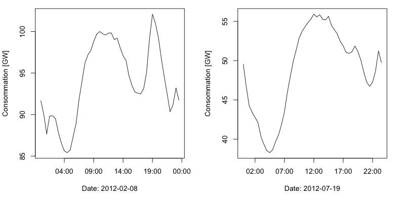 Figure 1 – Typical electricity demand profile (expressed in GW, a unit of power) for a cold winter day of 2012 and a hot summer day in France. Careful: the scales of the two graphs are very different! (Source: RTE French demand data)
In this particular example of Figure 1, the difference between the night-time trough and the daytime or evening peak is about 15 GW, and the difference is no more pronounced in winter. We are going to study the general distribution of these peaks over the year. These variations can be split into two parts, as is done in Figure 2: a downward variation (between the daily average and the trough) and an upward variation (between the daily average and the peak). Figure 2 gives the distribution of these variations in power for the period 2012-2018, a period over which they hardly changed. These variations are larger downwards (around 9-10 GW on average and up to 16 GW at most) than upwards (around 7 GW on average and up to 12 GW at most). Temperature (hot or cold period) has a fairly weak influence on the variations. For upward variations, the winter average is only a few hundred MW larger than during the warm season. This definition of the variations is simple and practical and will be translated into a modulation requirement in later posts. There are of course other ways of grasping this variability; one can for example consult [Heggarty2018] for definitions proposed at several timescales and the references therein.
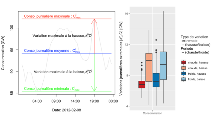 Figure 2 – A definition of the extreme upward and downward variations (left) and their distributions over the period 2012-2018 as a function of the time of year (heating period or not). Data source: RTE French demand.
Weekly variations can be linked to both causes mentioned in the introduction to this post. As regards the sensitivity of demand to temperature at the weekly scale, the arrival of a cold spell can raise demand by a few tens of GW in a day or two; we will study that phenomenon in the next section. As regards consumers’ schedules, it is essentially the variations between the weekend or days off and the working week that cause demand variations. In general demand is lower at weekends.
For these weekly variations one can carry out the same analysis as for the daily ones, by defining a downward (or upward) variation between the weekly average and the smallest (or largest) daily average demand. That is what is done in Figure 3, where it can be seen that these variations are larger downwards. This is explained by the fact that demand is lower only on weekend days, so the weekly average reflects rather a weekday.
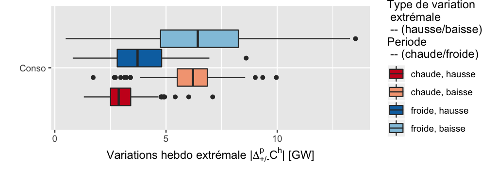 Figure 3 – Distributions over the period 2012-2018 of the extreme upward and downward weekly variations as a function of the time of year (heating period or not). Data source: RTE French demand. The weekly variation is built from daily average demand (see text).
Within a year, the largest variation is the seasonal one. The peak can exceed 100 GW in winter, as during the 2012 cold spell, whereas in summer it is around 50 GW. The existence and the size (almost 50 GW) of the difference between these winter peaks and the summer ones is mainly due to the sensitivity of demand to temperature. In winter, the colder it is the more electricity we consume: this is what is called thermosensitivity, on which I will give more detail in the next section.
Sensitivity of demand to temperature: defining thermosensitivity
Thermosensitivity quantifies how demand varies with temperature. Figure 4 shows this relationship between average daily French demand and average daily temperature. For temperatures below 15°C it is quite well described by a straight line. The slope of that line gives the additional MW of demand caused by a 1°C fall; that is how thermosensitivity is quantified. Below the threshold temperature (here 15°C) demand depends on temperature, and this threshold is therefore sometimes called the “heating temperature”. As a first approximation one can think of it as the outdoor temperature at which, on average, French households start heating with electricity.
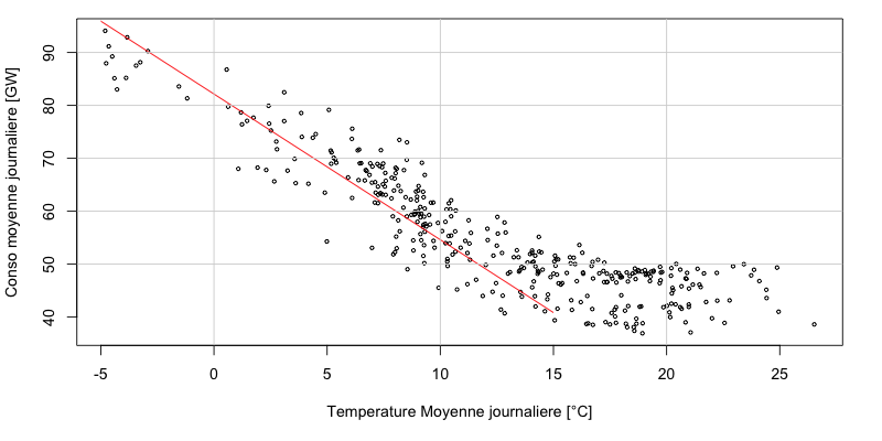 Figure 4 – A definition of thermosensitivity: the slope of the linear regression line between the daily average of demand and that of temperature, over a temperature range where the relationship is linear. Here on 2012 French demand data (source RTE) and with temperature data obtained from the spatial weighting of weather stations proposed by RTE.
Several definitions exist, but all rest on a linear model between electricity demand data and a temperature, for a well-chosen subset of the observations. Here that subset consists of the data for which the temperature is below 15°C, but it can also be defined by dates delimiting a period, or by a combination of the two. Demand here is a daily average, but it can also be taken at the daily maximum or at a specific hour. There are several ways of defining a national temperature. You can test different definitions of thermosensitivity using the shared code and data (see below the summary). Thermosensitivity is ultimately the slope of the linear regression line and is therefore measured in GW/°C.
The sensitivity of electricity demand to temperature differs across countries. In some countries there is also a warm temperature above which demand again depends on temperature, because of air conditioning. That is the case for instance in the United States or Italy, or in a few very particular places in France. At the scale of France there is no summer thermosensitivity. Between these temperature ranges (“heating temperature” and “cooling temperature” if it exists) demand is relatively independent of temperature. In some municipalities of southern France, locally, the effect of summer thermosensitivity combined with summer migration can mean that the local annual demand peaks occur in summer.
For winter in France, thermosensitivity was around 2.3 GW/°C (the equivalent of two nuclear units per degree) in 2013. The no-heating temperature is around 15°C. The linear relationship between demand and temperature explains why there can be a difference of almost 50 GW between demand on a summer day and demand on a very cold day when the national average temperature falls below -5°C, as happened in 2012. Figure 5 illustrates this phenomenon in different countries; it is very pronounced in France: European thermosensitivity, of the order of 5 GW/°C, is almost half French. This is essentially due to the use of electric heating, which is for now a French specificity. In the context of the energy transition we will tend to use electricity more and more as a heating means, but also to consume less thanks to efficiency.
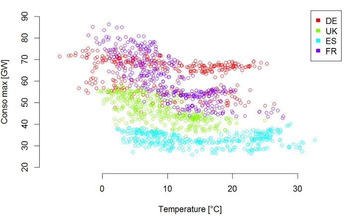 Figure 5 – Thermosensitivity of four European countries (Germany, United Kingdom, Spain and France); the daily demand peak is plotted against national temperature for the year 2015. Temperature data are obtained from the MERRA (NASA) database and demand data from ENTSOE.
Taking a daily average temperature and a daily average demand is preferred here to studying hourly variations. It avoids incorporating effects linked to consumers’ schedules (the extra demand at 7 p.m.) that are not caused by temperature but are correlated with it. Moreover, while the daily average temperature has a large influence on daily average demand (more than 2 GW/°C), what intra-day variations add to that dependence is smaller. To be more precise, if one studies the variables:
- X: the difference between the daily demand peak and the daily average
- and Y: the difference between the temperature at the time of the peak and the daily average temperature
one obtains a weak correlation between them and a linear regression slope of around 0.2 GW/°C (therefore much smaller than the 2 GW/°C), with no real evolution since 1996. The code made available for this post reproduces this analysis. We will come back to this point when we discuss the main cause of thermosensitivity — electric heating — and the thermal inertia associated with that end use.
Past evolution of thermosensitivity in France.
Annual electricity consumption since the creation of EDF in the aftermath of the Second World War grew by almost 5 TWh/year until the mid-1990s. That growth is linked to economic growth and to changes in the French way of life. These increases are more related to developments in the residential and service sectors than in industry, but we will discuss sector-by-sector developments in another post. That growth then slowed until the 2008 crisis, after which no significant increase has been detected so far.
During the years 2000 to 2012, however, even as annual consumption was slowing, a striking phenomenon occurred: the annual demand peaks increased a great deal. It is not easy to say how far this phenomenon is new, because hour-by-hour demand data before 1996 are not made available by the transmission system operator RTE. The peaks grew twice as fast as average demand, which corresponds to an increase of about 30% in 10 years, i.e. roughly 2 GW per year (Figure 6).
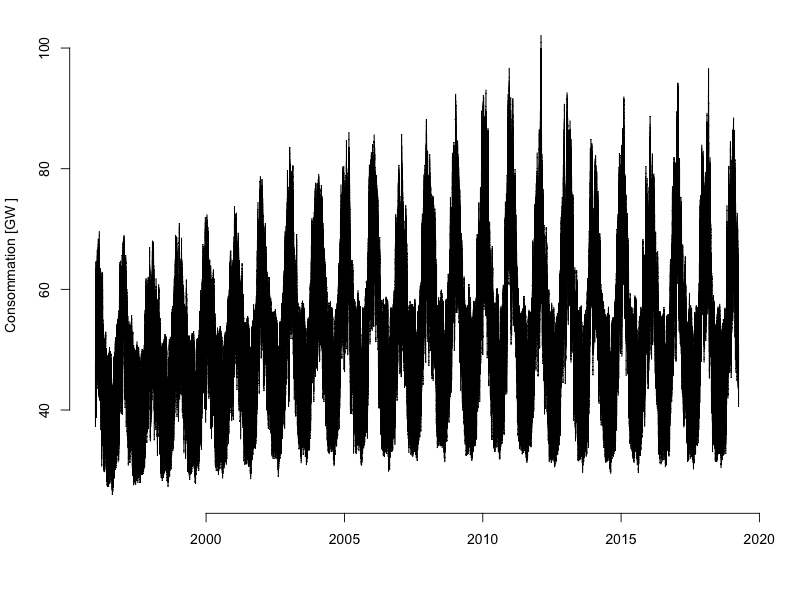 Figure 6 – French hourly demand from 1996 to 2019. Between 2000 and 2012, while annual energy consumption stagnates, an increase of about 30% in demand peaks is observed (Source RTE).
Thermosensitivity is almost entirely responsible for the increase in the peaks, since it tripled between 2000 and 2012, rising from 0.8 GW/°C to 2.4 GW/°C. That corresponds on average to more than 0.1 GW/°C extra each year. A temperature a little less than 13°C below seasonal norms caused a demand increase of 10 GW in 2000 and of the order of 30 GW in 2012. Thus the slight increase in annual consumption and the severe cold of 2012 explain almost entirely the evolution of the peaks presented in Figure 4. Figure 7 illustrates how the thermosensitivity phenomenon evolved from 2000 to 2012. One can also note that demand peaks are increasingly a direct consequence of temperature variations (the variance explained by the linear regression has been around 70% in recent years).
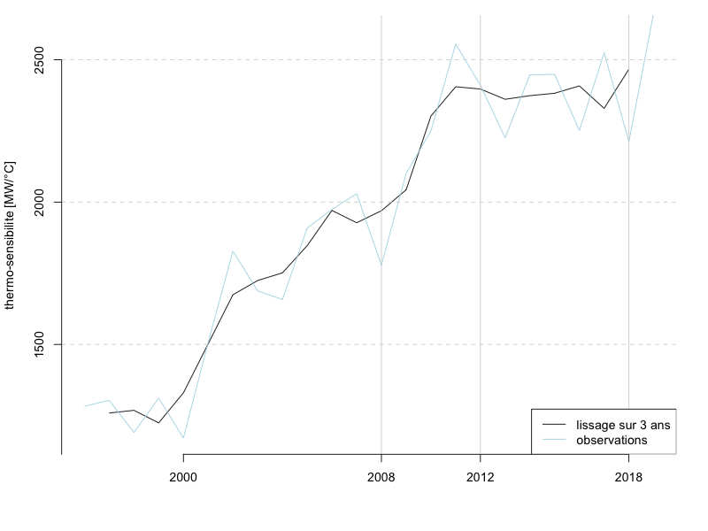 Figure 7 – Evolution of the thermosensitivity of French electricity demand over 20 years (from 1996 to 2019), 100 MW/°C more each year: slope of the relation “daily average demand” = f(daily average temperature).
We therefore observe a substantial increase in thermosensitivity. That increase appears to have started in 2000, but hourly demand data before 1996 are missing from this analysis. One can nevertheless think that the phenomenon of the years 2000-2010 is new, in the sense that the evolution of annual electrical energy consumption since 1970 has undergone a progressive slowdown. The trend in thermosensitivity is not confirmed by the years 2012-2018 (see Figure 7). It is interesting to try to understand, on the one hand, the consequences of this thermosensitivity for the cost of the power system and, on the other, what lies behind its past and future evolution, so as to model it properly in a foresight exercise. That is what we will do in later posts. As regards future developments, in a context of energy transition, they will be driven by one upward factor, the electrification of heating, and one downward factor, the improved efficiency of heating systems and building insulation. We discuss this in this post.
Conclusion
We have analysed the variations of demand at several timescales and according to several causes. We have given a definition of thermosensitivity — a simple concept, used for a long time by French electricity network operators (transmission and distribution) and for even longer by gas operators. We will have the opportunity to come back to it in future posts. In particular we will study the causes of thermosensitivity (essentially electric heating), as well as the consequences of the various forms of variation for the operation and planning of the power system. We will also study the variability of renewable generation and show how it too affects the power system: its operation and its sizing.