The code and data used to produce the graphs of this post are made freely available.
Describing a power system
Installed capacity and annual energy consumed.
On a territory (an island, a country or a continent) various kinds of electricity generation and storage are combined, and the whole they form is called the electricity generation mix. If the transmission and distribution network is added — which we will discuss in another text — we then speak of the power system. The electricity generation mix in France is composed essentially of nuclear and hydro plants, but it also includes gas plants, wind turbines, solar panels, tidal plants, and so on. The first two quantities one must learn to distinguish in order to grasp a country’s electricity generation mix are, on one side the annual energy produced — a “final” energy (as opposed to primary energy), most often expressed in TWh (or GWh, MWh, kWh) — and on the other the installed capacity, given in GW (or MW, kW). As we shall see in Section 3, the interest of describing a power system through installed capacities and produced energies is that these translate quite simply into economic costs and greenhouse gas (GHG) emissions. The graph below shows the split between capacity and energy for the various means of generation in France and Germany in 2018. Generation is grouped into broad classes according to the energy source used: nuclear, gas, oil, coal, wind, solar PV. We have gathered generation here under broad classes (wind, PV, nuclear, gas, coal, etc.) behind which lie important variants that we will detail shortly, with respect to technical capabilities, costs and environmental impacts.
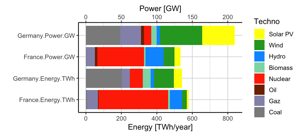 Figure 1 – Energy produced per year and installed capacity for different classes of generation in France and Germany in 2018. Dispatchable generation is to the left of the green zone; strongly carbon-emitting generation is to the left of the red zone (Oil, Gas and Coal). Data source: ENTSOE [1]
Dispatchable and non-dispatchable installed capacity
Installed capacity does not have the same value depending on whether it is dispatchable (gas, coal, nuclear, hydro) or relates to non-dispatchable generation (wind, solar PV) whose availability is not the result of a choice. Wind turbines and solar panels can only produce when there is wind or sun. In France dispatchable capacity is around 110 GW, whereas in Germany it is slightly lower, around 100 GW (these figures can be read on Figure 1 by totalling the installed capacities of the generation to the left of the blue hydro zone). This dichotomy is useful but a few nuances must be mentioned. A dispatchable generator never has 100% availability, because of maintenance requirements or certain operating constraints; but the maintenance behind the corresponding unavailability is most often the result of a choice that can be usefully optimised. That is the case, for instance, in France with nuclear, whose maintenance is optimised so as to adapt generation to the seasonal variation of demand caused by its thermosensitivity, as we have already discussed [2]. Part of run-of-river hydro is only partly dispatchable (with flexibility over a few tens of minutes). Non-dispatchable generation can be partially controlled, for instance by regulating downwards to manage a network constraint or a generation surplus on the system. That is what is sometimes called generation shedding, or curtailment.
Dispatchable capacity gives an order of magnitude of the maximum instantaneous demand that can be covered, but this question requires a more complex analysis taking into account other factors, such as, on one side, the maintenance requirements of dispatchable plants and the reserve requirements of the power system, which reduce the available dispatchable capacity, and on the other, the variations of demand jointly with those of intermittent generation, and the existence and availability of storage, interconnection and flexible demand, which can lower the dispatchable capacity requirement. It is not necessary at this stage to understand what lies behind all these terms; it is an important issue to which we will return. In France, during the very cold winter of 2012, we covered a demand of 110 GW.
Examples of electricity mixes around the world
The place occupied by a means of generation can be described in terms of installed dispatchable capacity, or in terms of annual energy produced. These two things are generally different. For example, nuclear contributes about 3/4 of electrical energy production in France but represents only a little more than half of dispatchable capacity (with 63 GW installed). Conversely, still in France, dispatchable hydro capacity holds an important place in capacity terms (of the order of 25 GW) but much less in energy terms. In Germany, wind and solar have a large installed capacity representing half the mix in capacity terms; these are non-dispatchable capacities that represent less than a third of the energy produced. But we shall see that the ratio between installed capacity and energy produced is relatively stable within a technology (that is the capacity factor, discussed in the next section). We therefore give in Figure 2 a description of the volumes of electricity produced by different technologies for different countries around the world.
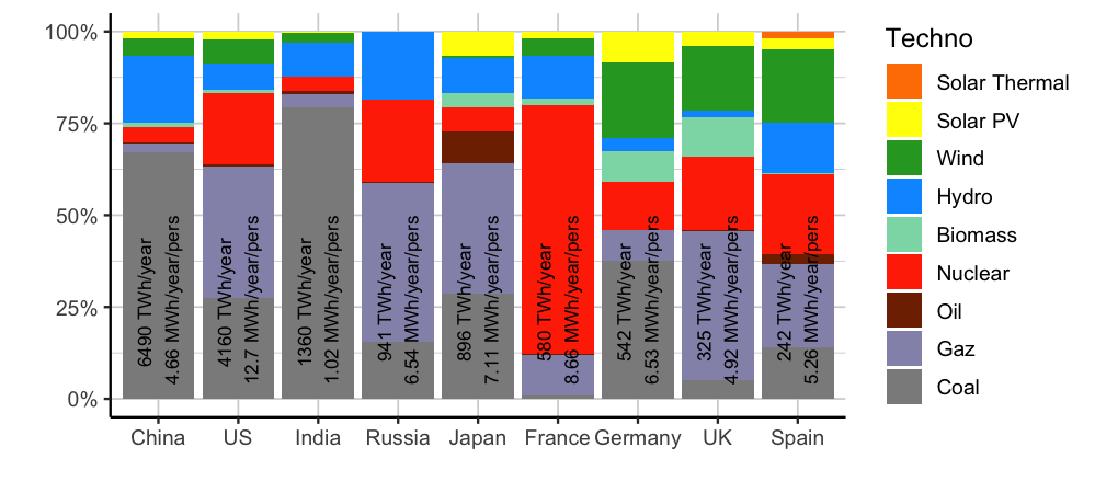 Figure 2 – Annual (electrical) energy produced in 2018 by country and by technology.
The data have varied origins but are all public; my work was to gather them for you in this document. Note that China therefore has an electrical energy production 10 times larger than Germany, which itself has a production twice as large as Spain. It is in France that low-carbon generation is largest, but Spain, Germany and the United Kingdom have a significant share of low-carbon generation.
Capacity factor
Definition
One goes from the installed capacity of a plant or a group of plants to an annual energy through the capacity factor, an essential element for describing the generation of the electricity mix. It is defined as the energy produced over a given period (an hour, a month, a year, etc.) relative to the energy that would have been produced by running at full output the whole time. The annual capacity factor is expressed either as a proportion or as a number of annual hours (obtained by multiplying the proportion by the number of hours in a year: 8760). Writing $E$ for the annual energy produced in TWh/year and $P$ for the installed capacity in GW, the annual capacity factor is given by:
\(FC=\frac{E}{P\times 8760 \times 10^{−3}}=\frac{E}{P\times 8.76}\)
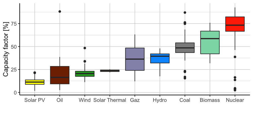 Figure 3 – distribution of capacity factors for different technologies over the period 2008-2018 and across the countries considered in Figure 2. These distributions are shown as box plots: the rectangle contains half of the values and the solid line 90% of the values; the points are extreme or outlying values relative to the other observations. One point represents the capacity factor of a whole fleet for a whole year in one country.
Figure 3 shows the distribution of the capacity factors of the different technology classes over the period 2008-2018 and across the countries considered in Figure 2. What is shown here is therefore not the capacity factors of individual plants but those of coherent groups of plants in different countries and for different years. These values are not weighted by the size of the different countries, and one cannot say that the chosen countries are exactly representative of the diversity that exists in the world; these values are therefore given as an illustration, mainly to show the range of possible values and the trend by type of generation. We will now give a few explanations about where these values come from.
Figure 3 – distribution of capacity factors for different technologies over the period 2008-2018 and across the countries considered in Figure 2. These distributions are shown as box plots: the rectangle contains half of the values and the solid line 90% of the values; the points are extreme or outlying values relative to the other observations. One point represents the capacity factor of a whole fleet for a whole year in one country.
Figure 3 shows the distribution of the capacity factors of the different technology classes over the period 2008-2018 and across the countries considered in Figure 2. What is shown here is therefore not the capacity factors of individual plants but those of coherent groups of plants in different countries and for different years. These values are not weighted by the size of the different countries, and one cannot say that the chosen countries are exactly representative of the diversity that exists in the world; these values are therefore given as an illustration, mainly to show the range of possible values and the trend by type of generation. We will now give a few explanations about where these values come from.
What influences the capacity factor
Several elements of different natures can influence the capacity factor of a means of electricity generation:
The weather — Solar PV generation depends on irradiance, wind depends on the wind, and run-of-river hydro depends on water availability and therefore on rainfall. Moreover, we have already seen that temperature influences demand and therefore also influences the generation set against it. Technical operating constraints — Let us give a few examples. The unavailability of nuclear plants for refuelling, which is about one month every year, two months every three years and three months every ten years. For nuclear plants on rivers, the flow rate and temperature of the water can be limiting, so drought periods are problematic — a real difficulty in the context of climate change. For hydro, the stock in our large dams, or respect for the use of watercourses for tourism or for the flora growing there, can be limiting. Flow constraints on the electricity network can require part of the generation to be limited locally for certain hours; that is the case fairly often today in northern Germany, where a large quantity of wind turbines is concentrated that is not well enough connected to the south of Germany. The cost structure of generation – We shall see that the costs of a generation technology can be broken down into fixed costs, which appear as soon as a plant is built and kept in operation, and variable (or marginal) costs, which appear only when the plant is producing (essentially fuel costs). The relative importance of these two cost items for a given technology affects the role it will play in the electricity mix to satisfy supply-demand balance (baseload vs peaking). For example, some plants installed for their low investment cost (such as certain gas plants) run infrequently because they have a high marginal cost and are therefore used only when the rest of the electricity mix is not sufficient to cover demand. They are installed nonetheless because their capacity cost (in €/kW installed) is low. These are called peaking plants. At the opposite end, nuclear has a low variable cost and a high investment cost; it is used as baseload and its capacity factor must be as high as possible, essentially for economic reasons.
In a system, each means of generation can affect the capacity factor of the others through its economic characteristics; demand variability also affects the capacity factor. Note too that a low capacity factor is not in itself the reflection of a technical difficulty; rather it is the variability and non-dispatchability of generation that may be, as with intermittent renewables (wind/PV).
Nor is a low capacity factor the cause of low economic or environmental interest. Indeed, if a system A produces four times less energy than a system B at equal installed capacity, but system B is four times more expensive, the cost per unit of energy produced for A, all other things being equal, is the same as for B. That is why economic cost is often related to the energy produced [€/MWh], which a priori allows economic comparisons independent of the capacity factor. We will now formalise this remark a little and give quantifications both for the economic side and with respect to GHG emissions.
Energy and capacity: two factors explaining economic costs and GHG emissions
Installed capacity and annual energy produced — or equivalently installed capacity and capacity factor — make it possible to estimate quite well the economic costs of the electricity generation system as well as its GHG emissions.
Economic costs
The annual expenditure associated with a country’s electricity generation (in M€/year) is estimated by a linear relation (summed over the means of generation) of the form
\(\sum_i \alpha_i^{cout} E_i+\beta_i^{cout} P_i\)
Indeed, part of the costs is directly proportional to the energy produced ($E$ is expressed in [TWh/year]); it most often contains fuel costs, and these costs are called “marginal costs”, given here by $\alpha_i^{cout}$ and expressed in [€/MWh]. On the other hand, the installed capacity ($P$ expressed in GW) induces fixed costs of investment and maintenance, staff costs, taxes, and so on; some of these costs are paid only at the investment stage, others every year. These costs are proportional to the installed capacity and one practice is to bring them onto an annual basis: $\beta_i^{cout}$, expressed for generation technology $i$ in [€/kW/year]. Economically this part is often significant, but its importance varies across technologies: nuclear and renewables have high fixed costs but low marginal costs, whereas for gas, oil or coal it is rather the opposite. But within each type of plant there is a range of possible cases that we do not detail here.
Gathering all costs on a common and intelligible time basis is very practical; here we use an annual basis, as is often done in energy. This simplification can be the source of a few difficulties and misunderstandings that must be mentioned.
First, fixed costs do not arise uniformly over the life of the project. Three phases can be distinguished in a project. They are the same as for buying a house: a large sum of money is spent at the investment stage, then after a longer or shorter period the project moves into an operation and repayment phase. Throughout the project, equipment may have to be replaced as it ages; that does not mean the project is at the end of its life, just that some investments have to be renewed. Once the initial investment is repaid, the project moves into an operating phase without repayment; the investment is said to be amortised. That last period is often a period of returns to shareholders.
One consequence is that a given year’s expenditure does not always reflect past or future average expenditure. In Table 1 we give a few values for economic costs and GHG emissions; the cost of nuclear “brought back to 2018” does not include any investment cost, since the French plants are already amortised, and it therefore does not reflect a future cost of nuclear. To obtain that, the cost of refurbishing the current plants or of building new EPRs must be added. Conversely, the cost of solar PV has fallen a great deal over the past fifteen years, but since we are still paying for the plants installed at a very high cost before 2010, the cost indicated in Table 1 is much higher than the cost of the plants being installed in 2018. In Figure 4 we give investment expenditure in renewables; one can observe the peak in PV expenditure linked to very high subsidised tariffs before the 2010 moratorium, which still weigh today on the cost of electricity even though the sector is now far more attractive economically.
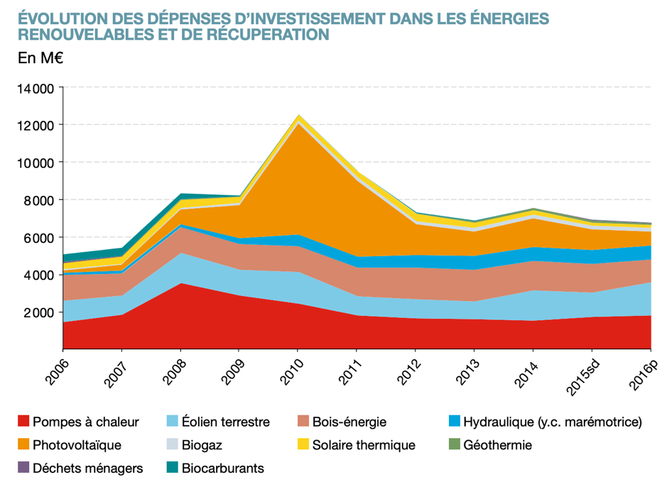 Figure 4 – Evolution of investment expenditure in renewable and recovered energies, see [3] p11. These are not subsidies but investment expenditure. One can see that spending on heat pumps, which we discussed in [2], has already been substantial for a long time and also peaked around 2008.
In every case annualisation raises a fundamental economic problem. It is a political and philosophical problem in some of its aspects. Indeed, it is impossible to compare objectively a sum of money spent now and a sum of money spent in the future. Consequently, one cannot simply divide an investment by the lifetime of the project to annualise the corresponding costs. The solution recommended by economists is to use the discounting model to make the revenues and expenditures of different years comparable: money spent in year $n$ has a value proportional to money spent in year $n+1$, the proportionality coefficient being $1+A$ where $A$ is the discount rate. We will present and discuss this method and its implications in a future post (here). Let us just note here that this method formally amounts to shortening the lifetime of projects in the revenue calculation, and all the more so as the projects have long lifetimes. This parameter has a very large impact on the results but is not easy to discuss; in Table 1 below we took a discount rate of 4%, which is rather a low rate but no doubt not the lowest possible. We will shortly make available an Excel file in which this rate can be changed.
GHG emissions and summary for the current French mix
It is important to recall that the environmental side does not reduce to GHG emissions, even though we restrict ourselves to them here. We are going to talk about wind, solar PV and nuclear, and these three energy sources, although low-carbon, raise a whole host of other problems (resources, land use, waste, accident risk, etc.) that we do not discuss here. We therefore insist, as we have in the past, that these energy sources are not neutral and that, as one often hears, “the best energy is the energy we do not consume”. As regards the GHG emissions of the power system, the largest part today results from the use of fossil fuels (gas, coal, oil) in the generation phase. It therefore corresponds to emissions directly proportional to the energy produced, which could be called “marginal emissions” by analogy with the economic side. Summing the corresponding emissions gives, in order of magnitude, what is given in the national low-carbon strategy (SNBC) document mentioned in the introduction of the heating post [2], namely about 20 MtCO2eq/year associated with the electricity generation sector, as can be seen in Table 1 below. In the same spirit as with the economic analysis, one can also account for the emissions linked to building the plant, or for those that are not “marginal emissions” but are linked to operating the plant. One then speaks of a life-cycle analysis: an analysis accounting for emissions from cradle to grave (from construction to decommissioning of the installation). That analysis is carried out over a perimeter that must be well defined (for instance here we do not account for the network), but it is then no longer necessarily compatible with a France-level analysis such as the SNBC’s, since it involves emissions from another year, in other sectors and very often in other countries too. While one must avoid forgetting something (such as emissions linked to production abroad), one must also avoid double counting (such as the production of steel to make the frame of a building that will serve electricity generation but which belongs to the steel industry and is used in the building sector before the building is used for electricity generation). Keeping this life-cycle analysis, the emissions of the electricity generation mix can be given by a formula very similar to the one given for cost.
\(Emissions[MtCO_2/an]=\sum_i \alpha_i^{emissions} E_i + \beta_i^{emissions} P_i\) This formula involves annualisation, and contains fixed and variable costs. Values are given in Table 1. At the scale of the mix, the fixed costs are much smaller than the “variable costs”, which correspond to emissions from burning gas or coal.
| Coal | Gas | Oil | Old Nuke | Wind | BioE | PV | Total | |||
|---|---|---|---|---|---|---|---|---|---|---|
| System | P | Installed capacity [GW] | 3 | 12 | 3 | 63 | 15,1 | 2 | 8,5 | 106,6 |
| E | Generation [TWh/year] | 6 | 31,0 | 2,0 | 400,0 | 30,0 | 10,0 | 10,0 | 489,0 | |
| FC | Capacity factor [%] | 22,83 | 29,49 | 7,61 | 72,48 | 22,68 | 57,08 | 13,43 | ||
| Cost | beta | [€/kW/year] | 110 | 90 | 60 | 200 | 150 | 110 | 350 | |
| alpha | [€/MWh] | 10 | 40 | 30 | 6 | 0 | 10 | 0 | ||
| Total | [€/MWh] | 65 | 74,8 | 120,0 | 37,5 | 75,5 | 32,0 | 297,5 | 48,1 | |
| [Billion €/year] | 0,4 | 2,3 | 0,2 | 15,0 | 2,3 | 0,3 | 3,0 | 23,5 | ||
| Emissions | beta | [gCO2eq/W/year] | 30 | 25 | 30 | 50 | 20 | 25 | 50 | |
| Marg | [MtCO2eq/year] marginal | 5 | 16 | 1 | 1 | 0 | 0 | 0 | 24 | |
| alpha | [gCO2eq/kWh] | 900 | 500 | 700 | 2 | 0 | 40 | 0 | 60 | |
| Total | [gCO2/kWh] | 915 | 510 | 745 | 10 | 10 | 45 | 43 | 57 | |
| [MtCO2eq/year] | 5,5 | 15,8 | 1,5 | 4,0 | 0,3 | 0,5 | 0,4 | 27,9 |
Table 1 – GHG emissions and average costs (roughly approximated) associated with the main French generation classes. The carbon content of electricity generation in France today is approximately recovered. 2018 data. Note that these emissions do not account for the impacts of the transmission and distribution network, nor for imports. Excel file. In the perspective of a low-carbon electricity mix, which could rest on means such as nuclear, biogas, PV and wind, the fixed part of emissions would be dominant. In such a context, or in a foresight exercise targeting carbon neutrality, one understands that it becomes important to account for where the generation equipment is manufactured. Note that here too, to be rigorous, emissions should be “discounted” (accounting for the fact that emissions now and emissions in ten years do not have the same impact on warming at a given horizon), but the effect is minor and to my knowledge is never taken into account in the literature.
Possible future “low-carbon” mixes
Some issues around the SNBC for the electricity generation sector
The French government is currently building a long-term vision of the energy transition through the national low-carbon strategy (SNBC), which targets carbon neutrality in 2050. That neutrality requires reducing marginal emissions from 20 MtCO2eq/year to 2 MtCO2eq/year. The emissions of the French generation mix are already low thanks to nuclear, and we are not that far from meeting this objective. One difficulty remains.
The major issue in France is linked to the ageing of the nuclear fleet. Even though plant lifetimes should no doubt be extended (or premature closures avoided, as with Fessenheim) by investing in refurbishment, most of the existing plants will very probably be shut down by 2050-2060. Given the time it takes to build a few GW, it would be very risky to have an entire mix with an average age above 60 years. That is the “cliff effect” the SFEN discusses in [4], Figure 4. In its response to the national low-carbon strategy, on the subject of the evolution of the power system, the Shift Project [0] recently recalled that “this system has a great deal of inertia and the ageing of the nuclear fleet will raise the question of its replacement by 2050”. So a new decarbonised electricity mix must be built, and that cannot be done overnight. It is not too early to get to work today. There are two broad alternatives for this, both delicate: building thousands of wind turbines and PV panels with the dispatchable capacity that goes with them, or building about fifty times Flamanville. Reality will probably be somewhere in the middle. In order to quantify the economic and GHG cost of these alternative mixes, we have used the previous equations here; the results are given in Table 2, which is also available as an Excel file in which you can modify the assumptions as you wish.
Another issue is the use of gas. It will be difficult to do entirely without the little gas remaining in the French power system today, because even if the energy volumes are very small compared with nuclear generation, the corresponding installed capacity is significant and useful in covering demand such as the thermosensitive heating demand we have already discussed [2]. Using nuclear at very low capacity factors would imply excessive costs. An important avenue on this point is biogas, which we have already discussed. We are talking about small amounts of energy (60 TWh of gas at most, so around 30 TWh/year of electricity from gas) but a large capacity, especially in the case of a renewable mix. Biogas will be much more expensive than natural gas, but the corresponding emissions are far lower (around 25 gCO2eq/kWh, even if this subject would deserve far deeper analysis; see the heating post [2]). In any case, the energy volumes involved here are small and, since the capacity cost of gas is low, the impact on the energy bill is limited.
| Future | Nuke | Future | Renew. | |||||||||
|---|---|---|---|---|---|---|---|---|---|---|---|---|
| EPR | Gas | Hydro | Total | Gas | Wind | Hydro | PV | Bat. | Total | |||
| System | P | Installed capacity [GW] | 63 | 6 | 25 | 94 | 35 | 170 | 25 | 90 | 10 | 330 |
| E | Generation [TWh/year] | 400,0 | 15,0 | 68,0 | 483,0 | 30,0 | 300,0 | 68,0 | 95,0 | X | 493,0 | |
| FC | Capacity factor [%] | 72,48 | 28,54 | 31,05 | 9,78 | 20,15 | 31,05 | 12,05 | X | |||
| Cost | beta | [€/kW/year] | 500 | 90 | 110 | 90 | 140 | 110 | 85 | 150 | ||
| alpha | [€/MWh] | 6 | 100 | 0 | 100 | 0 | 0 | 0 | 0 | |||
| Total | [€/MWh] | 84,8 | 136,0 | 40,4 | 80,1 | 205,0 | 79,3 | 40,4 | 80,5 | X | 84,9 | |
| [Billion €/year] | 33,9 | 2,0 | 2,8 | 38,7 | 6,2 | 23,8 | 2,8 | 7,7 | 1,5 | 41,9 | ||
| Emissions | beta | [gCO2eq/W/year] | 50 | 25 | 20 | 25 | 20 | 20 | 50 | 60 | ||
| Marg | [MtCO2eq/year] marginal | 0,8 | 0,8 | 0,0 | 1,6 | 1,5 | 0,0 | 0,0 | 0,0 | X | 1,5 | |
| alpha | [gCO2eq/kWh] | 2 | 50 | 0 | 11,08 | 50 | 0 | 0 | 0 | 0 | 23,88 | |
| Total | [gCO2/kWh] | 10 | 60 | 7 | 11 | 79 | 11 | 7 | 47 | X | 24 | |
| [MtCO2eq/year] | 4,0 | 0,9 | 0,5 | 5,4 | 2,4 | 3,4 | 0,5 | 4,5 | 1,0 | 11,8 |
Table 2 – Strongly nuclear or strongly renewable mix for 2050. Excel file.
Looking at these mixes, one understands that they have comparable costs. The alpha and beta values will be discussed in a later post (here). As for what could give rise to the most substantial discussion: nuclear is here below €85/MWh, i.e. less than plants such as Flamanville in France or Hinkley Point [5] in the United Kingdom, which are first-of-a-kind units, but a value closer to what would be obtained by applying the investment costs of the Taishan plant in China. PV and wind appear in Table 2 at prices around €80/MWh, which is less than projects built in the 2010s but much more than some projects being built today at between €50 and €60/MWh (see [6] for PV and [7] for wind). The discussion on this thorny and much-debated subject could be long, and the idea here is only to show that it is hard to imagine (short of really twisting the figures) that there would be a very large difference between the two mixes. Of course, the economic assumptions can be changed, and supply-demand balance discussed, to make one system or the other win; but the uncertainties at this horizon are large, and ultimately the issues and difficulties are not only economic and are very numerous, both for renewables deployment and for new nuclear deployment — we will come back to this. It seems that at the scale of the Earth (the scale to consider ultimately when it comes to meeting the challenges of climate change), these can take different forms. In many cases both forms of energy can play a role, which will no doubt depend a great deal on regions and countries. We do not think there is ground here to discredit either solution. In terms of GHG emissions for the French case, both systems are compatible with the SNBC, with “marginal” emissions falling from 20 MtCO2eq/year to less than 2 MtCO2eq/year in both cases.
Dispatchable capacity of the renewable mix
It is not possible to compare, economically or environmentally, a dispatchable generation technology such as nuclear with an intermittent one such as solar PV or wind. These technologies do not provide equivalent services. The appropriate methodology in that case is to compare a nuclear system with a renewable system plus sufficient back-up (biogas, storage, hydro, etc.), i.e. one that ensures supply-demand balance at any moment and at every point of the network. That is what is called the system cost, and it is what we give here in Table 2, even if it is a somewhat simplified version. We will discuss in another post whether the back-up proposed in Table 2 is sufficient for the renewable mix. For now we can give the following simple calculation: if 3% of the wind capacity installed at country scale is considered available 100% of the time, that gives (together with gas, hydro and battery storage) 75 GW of dispatchable capacity in the renewable mix. Further analysis will be presented to show that this capacity is sufficient, and that the 30 TWh/year of electricity from biogas are too. It must be understood that these systems are very simplified here, since one would have to account for interconnections with neighbouring countries, the possibility of demand-side management, the downward control of renewable generation (which we do account for in volume, by lowering the capacity factors of renewables in Table 2), the variants of each generation technology, the interactions with the gas network and with hydrogen systems. Note that the transmission system operator RTE is currently preparing a study on this subject. What we give here provides orders of magnitude concerning electricity generation but certainly does not aim to define a future mix. The only thing we want to illustrate is that the cost of the generation system depends far more on the energy produced than on the installed capacity: the renewable mix has an installed capacity almost 4 times larger than that of the nuclear mix, but comparable costs. In both cases the marginal GHG impacts are reduced satisfactorily (i.e. compatibly with the SNBC).
GHG emissions linked to construction, maintenance, etc.
Emissions linked to the construction phase of a plant, or to its decommissioning, remain. In the SNBC these emissions (and the associated beta values) must be reduced in the industrial, construction and transport sectors. The construction sector includes for instance concrete production; the industrial sector includes the extraction of iron or copper ore and the production of steel or aluminium — because these materials are heavily used here and produced with very carbon-intensive energy sources. The transport sector concerns the transport of raw materials, components and people. Over the perimeter of these “non-marginal” emissions, it should be noted that although both systems (nuclear / renewable+back-up) are compatible with the SNBC, the nuclear system is half as carbon-intensive as the renewable system. There are several reasons for this, but one important reason is the plant lifetime taken in the calculations (60 years for nuclear, whereas only 20 years are considered for wind turbines and PV panels). One can think that these durations will increase over time: many wind farms have now passed their 20 years of life, and feedback from experience — like that which allows the initially planned lifetime of the nuclear plants in place today to be extended — enables significant changes. Moreover, plants are often decommissioned for economic reasons that will no longer hold in a few years: new plants on the market perform better, and it is often better to build a new plant to obtain new subsidies on a site already secured than to keep an old plant running. Above all, the underlying question is the decarbonisation of industry. When one looks at the electricity sector, this issue does not seem very important because the associated emissions are low compared with current emissions; but in a decarbonised future the calculations and the optimisations with respect to these emissions will, we hope, be more thorough.
Conclusion
We have proposed tools for analysing electricity generation mixes simply, from installed capacities and annual energies produced. We have shown why the energy produced, more than the installed capacity, is the explanatory factor for GHG emissions and economic costs. We have recalled that an important issue in the context of the national low-carbon strategy is the renewal of the French nuclear fleet by 2050-2060. We have given orders of magnitude indicating why the caricatural “all renewable” or “all nuclear” systems have comparable costs for that renewal and are compatible with the national low-carbon strategy. Ultimately the issues are not only economic, and are very numerous both for renewables deployment and for new nuclear deployment — we will come back to this. It seems that at the scale of the Earth (the scale to consider ultimately when it comes to climate change), the problems raised by these two options can take different forms. In many cases both forms of energy (nuclear/renewable) can play a role, which will no doubt depend a great deal on regions and countries. We do not think there is ground in this text to discredit either solution. It should be noted that the clashes on this subject do not bode well for a simple transition of the French system by 2050. For now acceptability is a significant difficulty, on both sides in France, so the important thing is certainly not to believe that electricity is an infinite, perfectly clean or simple-to-deploy resource. In terms of GHG emissions for the French case, both systems are compatible with the SNBC, with “marginal” emissions falling from 20 MtCO2eq/year to less than 2 MtCO2eq/year in both cases.
When one looks at the emissions of the electricity generation sector, the part of those emissions linked to the construction phase of the plant, or to decommissioning, does not seem to be a major issue, because it is small compared with the current emissions of the electricity sector. For the nuclear system the corresponding emissions, related to the energy produced, are smaller than for the renewable system. But in a less carbon-intensive future, the calculations and optimisations with respect to these emissions will, we hope, be more thorough. In that perspective, accounting for the emissions of the industry and transport sectors, on which the construction of electricity generation equipment rests, will become more and more important. As regards industry, one thinks here of metal and concrete production and of raw material extraction. One can therefore imagine that one day, being compatible with the national low-carbon strategy will imply a certain provenance for the materials used in construction, minimising the associated emissions. In this post we have mentioned several subjects that will be the object of future posts: the evolution of the power system, the sub-classes of generation technologies (hidden behind the broad classes used here), the variability of renewable generation and the means of managing it, environmental impacts other than climate change, the computation of annualised costs (and the famous discounting), demand-side management, the SNBC in transport and industry, and so on.
Bibliography
[0] The Shift Project’s response to the SNBC
[1] ENTSOE Transparency Platform
[3] Key figures for renewable energies – 2019 edition. Graph p11
[4] Revue générale du nucléaire, Figure 4. November 2019.
[5] Tariff obtained for Hinkley Point in the United Kingdom 2019.
[6] Coûts et rentabilités du grand photovoltaïque en métropole continentale. CRE study, February 2019, on the responses to calls for tenders.
[7] Results of the third-quarter 2019 wind calls for tenders in France (CRE).