This post complements the “energy and capacity” post [PostPrec] but it can be read separately. It is probably even more natural to read this post first. We give a simple, fairly classical formula for computing the levelised cost of electricity. It rests on grouping costs into several categories: investment costs, operation and maintenance costs, and marginal costs. For each of the various means of generating electricity within the broad classes used in the previous post (nuclear, gas, coal, wind, solar, hydro), we give these different costs and some detail on the elements affecting the capacity factor. This also allows us to give orders of magnitude for the levelised cost and to recover the values used in [PostPrec]. In a previous post [PostPrec] we presented a way of modelling the economic and environmental costs of a power system from knowledge of the annual energy produced $E_i$ and the installed capacity $P_i$ of each means of generation $i$ in the system: \(\sum_i \alpha_i^{cout} E_i+\beta_i^{cout} P_i\) This allowed us to recover orders of magnitude for the cost of our current system and to assess it for 2050 for a strongly renewable system and a strongly nuclear one. Values for the coefficients $\alpha_i^{cout}$ (in [€/MWh]) and $\beta_i^{cout}$ (in [€/kW/year]) were proposed without explaining how they are obtained. The coefficient $\alpha_i^{cout}$ is called the proportional cost or variable cost. One also sometimes speaks of marginal cost, but in some communities that term is reserved for the variable cost of the last generator called upon at a given hour, i.e. the marginal cost of the power system. Here we are therefore talking about the part of the cost proportional to the energy produced for a given means of generation. As a first approximation, it depends on fuel costs, taxes and the efficiency of the installation. The discounted, annualised fixed cost $\beta_i^{cout}$ is obtained from economic data such as the discount rate, the investment cost and the annual operating costs, in a way we will detail in the first part of this post. This will let us introduce the LCOE (levelised cost of energy), which is widely used in the field. Moreover, we considered broad families of generation technologies: “nuclear”, “coal”, “gas”, “hydro”, “solar PV”, “wind”. Specifying the economic data and capacity factors for each family requires some detail on the diversity of existing technologies. In this second part, we will apply to each family the LCOE formula given in the first part.

Levelised cost (LCOE).

Introduction: discounting

When comparing the cost of electricity generation systems, two major difficulties must be faced. The first is economic: the heterogeneity of how expenditure is spread over time across families of generation technologies requires bringing all costs and revenues back to a single date to make them comparable. The second major difficulty comes from the fact that one cannot directly compare a MWh produced by a dispatchable generator with a MWh of must-run generation (e.g. wind, solar PV) — but we have already discussed this in our previous post [PostPrec].

To address the first difficulty, cost-focused economists and the engineers who develop projects have long used the discounting model. It rests on a single assumption that is simpler to understand and state than to discuss: the money $x_{n}$ earned or spent in year $n$ is worth more than the money $x_{n+1}$ earned or spent in year $n+1$. The extra value is $x_n r$, where $r$ is called the discount rate — indeed, it allows the value of money to be “brought up to date” from one year to the next. This model makes $x_{n+1}/(1+r)$ and $x_n$ comparable, but also, since $r$ does not depend on $n$, by recurrence, $x_{n}/(1+r)^n$ and $x_0$. By adding up the discounted expenditures and dividing by the energies produced, themselves discounted, one computes the levelised cost of energy, denoted $LCOE$. A formula is available here; in the next section we give an alternative form — nothing revolutionary, but it has the advantage of being compact and easier to handle.

We will not discuss more deeply what lies behind discounting here; it is a vast subject. Let us just note that $r$ is around 4-5% in publicly backed projects (that rate is then often framed by law) and rather around 8-10% for privately backed projects. That difference is mainly explained by the need to remunerate shareholders and the search for short-term returns in a private project. If $r$ equals inflation plus a rate of return on investment, then the LCOE corresponds to the purchase tariff that a project developer is likely to request in a call for tenders (except in the case of a contract for difference such as Hinkley Point, where the price is indexed on inflation, which must then not be included in the discount rate); see [Williams2019]. We defer a few elements of discussion around discounting to Appendix 1: accounting for the company’s own capital, inflation, the long-term interest rate, the return on capital, a company’s growth, banking fees, interest during construction, discounting and degrowth, and so on.

Project expenditure

To compute the LCOE, all the project’s expenditures must be listed, from the first euros spent before the plant is started up to the point where nothing more is earned or spent, after the shutdown, the decommissioning of the plant, its recycling and the treatment of waste. It is complex work, and the aim here is not to give an example of a detailed LCOE calculation but rather a simplified version allowing everyone to understand the important factors. In electricity generation (and in many other sectors) it is convenient to classify expenditure into 4 parts:

Note that, for the simplified LCOE formula that follows, all expenditures are either annualised (in the “operating cost” category) or brought back to the project start date, or brought back to the date of end of operation. There are two types of underlying assumption.

On one hand, this requires assuming that certain factors do not vary from year to year, such as the capacity factor or $C_F$ defined in [PostPrec]. That is obviously never the case, but if there is no asymmetry in the distribution of the coefficient in question year after year (e.g. a tendency towards a higher or lower capacity factor in the first years of operation), a mean value can be used without too many scruples. The capacity factor will often tend to fall over time in some installations, either through wear of the machinery or through an increased need for maintenance. Conversely, operating costs will tend to rise over the years. On this subject one can read the interesting discussion in [Williams2019].

On the other hand, when one speaks of a construction cost, a decommissioning cost or a waste management cost, there always lies behind it a series of expenditures occurring at different moments of the project, gathered together through discounting. Regarding construction cost, we discuss this in the Appendix.

Simplified formula

With the previous definitions, one can easily show that the LCOE of a given technology is expressed as a simple function of these parameters and of the capacity factor $FC$ ($P$ still being the installed capacity in GW and $E$ the annual energy produced in TWh): \(LCOE =\beta*\frac{P}{E}+C_M=\frac{\beta }{FC\times 8,76}+C_M\) where $ \beta $ is what may be called the “discounted average annual capacity cost”, expressed in [€/kW/year] and given by the formula: \(\beta = \frac{C_I}{L_{r}}+\frac{C_D}{(1+r)^{L}}+C_F\) This recovers the full-cost formula given in the introduction and used in [PostPrec], since for a technology $i$ the full cost brought back to one year is: \(LCOE_i*E_i =\beta_i*P_i+C_M*E_i=\beta^{cout}_i*P_i+\alpha^{cout}_i*E_i\) Here $L$ is the project lifetime, and $L_{r}$, given by the formula: \(L_{r}= \sum_{i=0}^{L-1}\frac{1}{(1+r)^i}=\frac{1+r}{r}(1-(1+r)^{-L}),\) is homogeneous to a lifetime that would be, as it were, (economically) shortened by “the effect of discounting”. We give in Appendix 2 a table of values of $ L_{r} $ as a function of $r$ and of the true lifetime $L$. What should be remembered about this “corrected” lifetime is that it is shorter than the true lifetime, and that the smaller $r$ is (close to zero), the closer $L_{r}$ is to $L$. Note that the simple formula proposed resembles the approach given by [NREL2018], and $L_{r}$ is close to being the inverse of what is called the CRF (capital recovery factor). $L_{r}$ can be given for the following emblematic cases:

One understands the extent to which large values of $r$ amount to mortgaging the future. Reality is obviously far more complex than what a discounting model can frame. Whatever the decommissioning cost $C_D$, its weight is almost always negligible because of discounting. That weight will be all the more negligible if decommissioning takes place over a very long period (as with nuclear, where waiting times are needed to let radioactivity decrease). In the tables of the next section, we give a few typical values of $ C_I $, $C_F$, $\beta$ and $C_M$.

Some detail on the diversity hidden behind these broad classes of generation

In this section we go through the broad classes of electricity generation and, for each of them, we discuss the different kinds of cost in order to give orders of magnitude for the LCOE. We do not discuss the cost of the power system here, and we refer the reader to our previous post [1].

Nuclear plants

As regards nuclear, one distinguishes several generations. The second generation is the one in operation today, built between the early 1970s and the late 1980s. The new plants being built today are third generation. Among the many technologies deployed commercially today (second and third generation), the two most important are boiling water reactors (BWR) and pressurised water reactors (PWR). A more exhaustive list is given in the link on generations. The fourth generation is planned for the coming decades (a pilot project has appeared in Russia, but it is not a molten salt reactor allowing waste reprocessing); several proposals aim, through significant technological changes, at plants that no longer use the same fuel but a much less rare form of uranium, that allow part of the existing long-lived waste to be reprocessed, that present no runaway risk, and that can more easily modulate their output without efficiency losses (we will come back to the modulation of current nuclear plants in a later post, because some things are possible but not everything, and it is an important subject). In France the Astrid research project, recently abandoned, was in this line, but internationally other projects continue in this direction. Finally, another generation of nuclear will arrive with fusion. On how nuclear plants work, I refer to the Le Réveilleur videos (a YouTuber doing documented and accessible work whom I will cite often).

In terms of costs, transparency in France has improved a great deal through a continuous analysis by the Court of Auditors over the past 10 years, sanctioned by at least 5 reports CDC2012, CDC2014, CDC2016, CDC2019, and CDC2020. Yet no detail is given on investment costs, and this lack of transparency is a peculiarity of nuclear that makes any investigation difficult. In the table below I give some investment and operating costs in France with the associated sources; most of the figures come from [CDC2014], tables p11, 14 and 24. Some values and discussions are supplemented by other reports.

With a capacity factor of 75%, the following costs can therefore be assessed. We lack information to cost the operation of the EPR, but these elements give orders of magnitude and we will take a value of €175/kW/year. What is called “economic rent” in current nuclear is not a cost. For the EPR, that shareholder remuneration is recovered if a higher discount rate of around 8-9% is taken instead of 4-5%. At that discount level we obtain for Hinkley Point C an LCOE of around €120/MWh. In order of magnitude, that corresponds to what was obtained by EDF from the British, £92.5/MWh (in 2012 currency) (it is a contract for difference, CFD; the tariff is indexed on inflation, so inflation is not included in the discount rate calculation — see Appendix 1 — but the real rate of return expected by EDF is announced at around 9%). One can therefore note that historical nuclear electricity gives us an average generation cost in France of around €50/MWh, but that in future, with the refurbishment programme or with EPRs, these costs will necessarily rise. Looking at the current cost without rent and at the cost of Flamanville, it seems possible that even with a series effect we would see a doubling of the cost of energy production. The main reason is that current nuclear has long been amortised and that its ageing requires new investment (either for refurbishment or for replacement). One can add that the current plants were built in a different economic context, with very high inflation in a period of growth, centralised planning, and project management with far less subcontracting. That said, even at €80/MWh, one can say that nuclear energy — which has the great advantage of being both dispatchable and low-carbon — has costs that can be kept under control, provided its financing is guaranteed by the State (to obtain low discount rates) and that it is deployed massively (scale effects being necessary to lower costs and maintain skills).

System	CAPEX €/kW	proportional €/MWh	Other €/kW/year	Lifetime	discount rate	LCOE
Current fleet average without rent	0	6	201	x	5%	36
Current fleet average with rent	0	6	331	x	5%	56
Refurbishment phase 1 with rent	0	6	352	x	5%	60
Refurbishment phase 2 with rent	0	6	411	x	5%	68
Flamanville, Hinkley Point (EPR)	7000	6	175	80	5%	84
Taishan (EPR)	3500	6	175	80	5%	58
Flamanville, Hinkley Point (EPR)	7000	6	175	80	9%	120
Taishan (EPR)	3500	6	175	80	9%	76

Gas, oil and coal

Plant types and investment costs

For gas (and oil), several broad categories of plant are distinguished. The most elementary is the gas turbine (OCGT, open cycle gas turbine in the case of gas), in which the gas or oil is mixed with air and sent under pressure into a turbine where it ignites. The principle of the OCGT is very close to that of a jet engine. In the OCGT the heat of the exhaust gases is lost, but it can be recovered in various ways. A first solution is to heat water (in a sort of large boiler) whose vapour will drive a second turbine connected to that of the gas turbine. That is what is called a combined cycle (CCGT for combined cycle gas turbine). The efficiency of a CCGT is therefore better: it can rise to around 55% (there is even a record of 64% held by the Bouchain plant), whereas that of the OCGT is limited to around 35-40% (except for very particular technologies using supercritical fluids). The installation cost of a CCGT is higher, and it takes a few hours to start, whereas the OCGT needs no more than 30 minutes. Another way of using the exhaust gases of the gas turbine is to extract the heat directly for another application (district heating, greenhouses, etc.); that is what is called cogeneration. In that case the overall efficiency of the installation is better, but the use of the turbine is somewhat subordinated to the heat requirement: one is obliged to produce when it is cold, and not necessarily only when electricity is needed.

In a coal plant one generally heats water by burning coal; the pressurised steam thus generated is sent into a turbine that produces electricity. For coal-fired electricity generation several technologies exist, more or less efficient depending on the pressure level used during combustion. The corresponding efficiencies can vary between 30 and 50%, and the environmental impacts (CO2, SOx, NOx, heavy metals, etc.) also vary a great deal with the quality of combustion. The coal industry highlights the increased efficiency of its new plants, which send “supercritical” fluids into the turbine, as well as the sequestration of carbon captured at the stack (able to capture up to 90% of CO2 emissions). Yet coal remains at present one of the most polluting means of generating electricity, on many counts.

System	Efficiency	CAPEX €/kW	Fixed O&M €/kW/year
Gas – OCGT	35%	500	15
Gas – CCGT	54%	900	20
Coal – Subcritical	40%	1200	45
Coal – Supercritical	45%	1400	40
Coal – Ultra-Supercritical	50%	2000	30

Table 1 – Gas- and coal-fired electricity generation, their efficiency and the corresponding investment cost. Source for coal and gas: [Cost2013]; additional source for gas: U.S. Energy Information Administration [EIA2016] Electricity generation from biomass is fairly similar to what is done with coal: combustion of the biomass to heat water and drive a steam turbine. The quality of combustion, the renewable character and the environmental impacts depend a great deal on the biomass used, its nature and its origin; they can be acceptable when waste is used, or biomass that is local and immediately replaced, but also very bad when, for example, forests are cut on the other side of the world without anything being replanted.

Fuel costs

One generally distinguishes electricity produced from low-quality coal — such as lignite — from that produced from black coal. There is a great variety of coal types linked to different degrees of coalification. They differ notably in their moisture content, carbon content or calorific value. There is no single internationally accepted definition allowing coals to be classified precisely, but a classification and some explanations are found in ADEME’s Base Carbone [ADEMEGES]. Lignite is less dense, its combustion is poorer and therefore more polluting (not really in terms of GHG emissions, though — see the table below), and its transport (related to the energy it delivers) is more costly. It is often extracted in open-pit mines, which may have a short-term economic advantage but certainly not an environmental one. Lignite therefore continues to be exploited where it is a local resource, for cost reasons and sometimes to preserve a local economy. Germany has an important lignite resource on its territory, used for half of its coal-fired electricity. Economically, at a cost of €5/MWhth (table below) that gives, for a plant with 40% efficiency, a proportional cost of less than €15/MWh. With such a proportional cost, these plants run as baseload rather than as peaking plants. With better-quality coal, imported for Germany or France, one ends up with a proportional cost between €20 and €25/MWh. A carbon tax of €1/tCO2 adds roughly €1/MWh here; one clearly sees that without a carbon tax coal still has a promising future.

Products	Emissions	NCV	Share			Cost [$/ton]		Cost [€/MWhth]
	gCO2eq/kWhth	(kWhth/kg)				2017	2017	2017	2017
		(TWhth/Mt)	US	World	DE	US	DE	US	DE
Anthracite (hard/black coal)	384	9 to 10	1	14	-	93		8.8
Bituminous	374	5 to 9	46	76	-	55	50	7.7	7
subbituminous	377	4 to 5	45	-	-	14		3
Lignite (brown coal)	393	2 to 3	9	14	100	19	20	5	5

Table 2 – different kinds of coal. Sources: U.S. EIA [4] and ADEME [ADEMEGES].

For gas, a distinction must be made between liquefied natural gas (LNG) and non-liquefied gas. Non-liquefied gas is transported essentially by pipeline, so its price is homogeneous within an interconnected network (even if price differences can exist when interconnections are saturated, as sometimes happens between the north and south of France). Liquefied natural gas is transported by ship and then delivered worldwide by truck; it is more expensive but its price is homogeneous across the globe and therefore more stable. The main advantage of LNG is to deliver gas to regions without gas transport infrastructure. Nevertheless, the energy-intensive liquefaction processes strongly worsen its carbon balance. (Black) coal and gas therefore have prices that vary in time and space and are linked to oil prices. A representation is given in Figure 1. All peaked in 2008 and then fell substantially. They are today in a deep trough linked to the COVID-19 crisis. 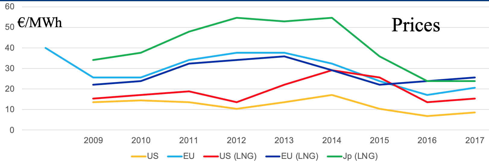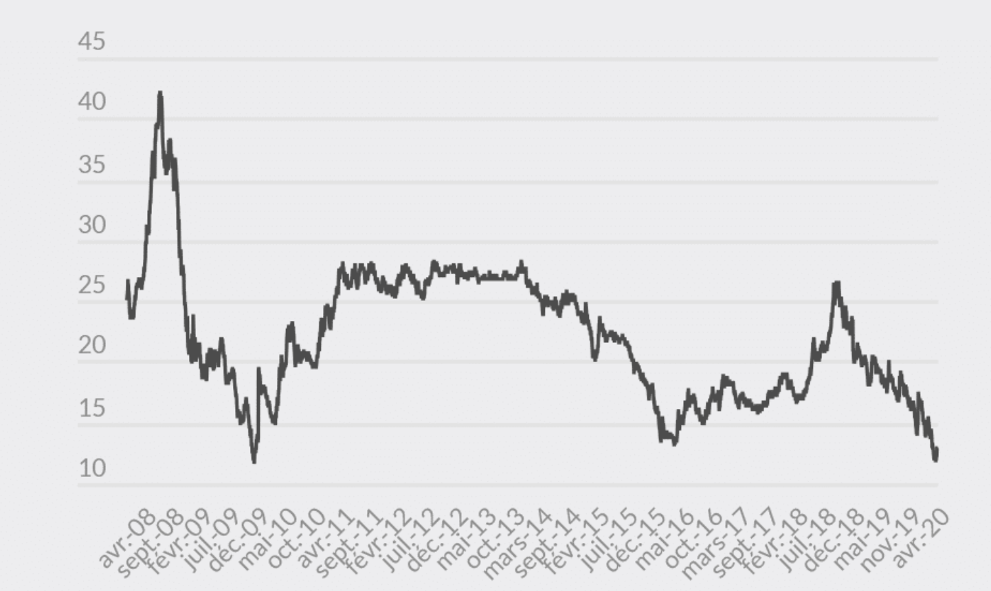Figure 1-a – Evolution of gas prices since 2009 (with 2008 for Europe to illustrate the peak), annual average data, then EEX Europe data extracted in 2020.

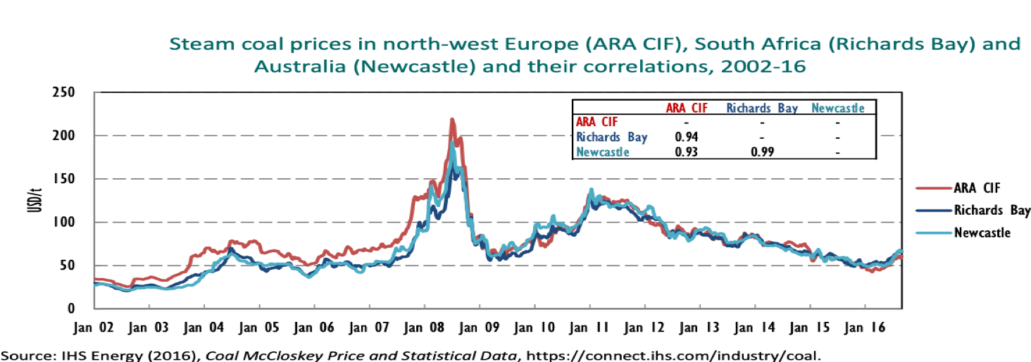Figure 1-b – Evolution of coal prices.

Hydro plants

The principle of a hydro (or hydroelectric) plant is to pass water through a turbine to produce electricity. There is a great diversity of hydro plants, which can be grasped by looking at the capacity and type of the turbine, the size of the upper reservoir if there is one, and possibly the presence of a pump and an upper reservoir. The delivered capacity can range from 22 GW for the Three Gorges Dam in China to a few MW for small hydro, a few kW for micro-hydro at the bottom of your garden, or even a few watts to a few hundred watts for pico-hydro sometimes used in water networks. There are many types of turbine, whose characteristics vary with head and flow; the three most used today are Kaplan, Francis and Pelton turbines. Note the existence of systems allowing the turbine to run at variable speed, and the existence of a pump to send water back up to the upper reservoir. On the other hand, one distinguishes “run-of-river” hydro, which uses a river or a small stream without a storage reservoir, from a large alpine valley dam that collects a low flow but can hold several days of full-output generation in stock. Run-of-river in some large plants of the Rhône valley nonetheless allows output to be modulated over one or two hours. Some dams are equipped with pumps that send the water back up and thus play a role of electricity storage; these are called pumped storage plants (Station de Transfert d’Energie par Pompage, STEP in French). In France we currently have a little less than 5 GW of pumped storage, some with storage capacity of up to several days (72 hours for the largest). The French hydro resource is close to saturation, but some large dams could be equipped with pumps to increase the available storage capacity — about 2 GW more is mentioned. There is also a resource of micro pumped storage, which we will discuss later when storage is addressed more precisely.

IRENA2012 is an interesting source of observed costs. Investment costs (CAPEX, capital expenditure) for systems with storage (with an upper reservoir) vary essentially with earthworks and the quantity of concrete to be poured. The turbine and the water supply (penstocks) cost around €400/kW where the complete project comes to between €900/kW and €3000/kW. The price rises slightly for small systems and generally falls with head. Operating cost is of the order of 2% of CAPEX each year, i.e. around €30-60/kW/year. The capacity factor depends greatly on the water availability of the site; it can vary from 25% to 90% and will therefore be one of the main elements influencing the LCOE.

Solar plants

For solar photovoltaics it is relevant to distinguish plant sizes: large ground-mounted plants occupying several hectares, plants on the roof of a shopping centre or over a car park (called “shade structures” for the shade they give to cars), and small plants of a few kW on the roof of a house. For large plants one must distinguish those with tracking systems (single-axis or dual-axis systems that follow the position of the sun in the sky to maximise output) from those without.

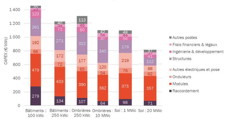
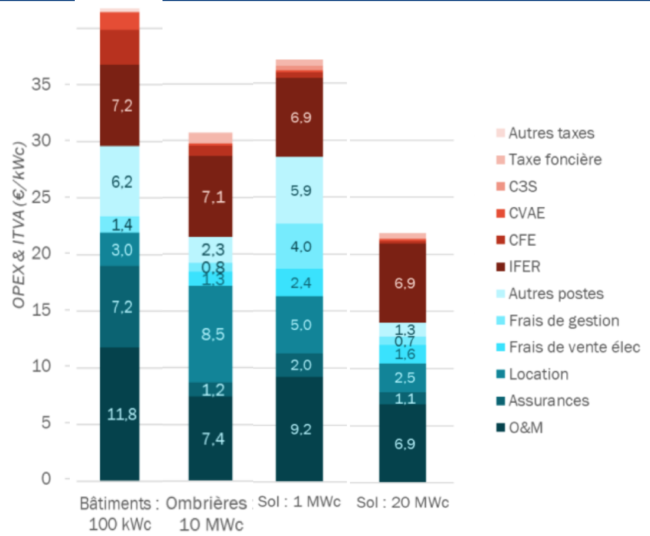Figure 2 – Breakdown of the average costs (CAPEX and OPEX) observed in the CRE calls for tenders, study published in February 2019, [CRE2019]. Finally, one of the factors that essentially determines the capacity factor of a photovoltaic system is the location of the plant. A plant in southern Spain will produce more than one in northern Germany, and above all its winter/summer variability will be much smaller — but we will come back to all this quantitatively when we discuss the variability of these generation technologies. Environmentally, where the panels are built (and the electricity mix used to run the machines that produce the panels) can also matter. For large PV plants, LCOEs between €45 and €65/MWh are found, which corresponds to the orders of magnitude found in the responses to the calls for tenders run by the French energy regulator (CRE), as in 2020 [CRE2020PV], where the average price of selected projects was around €60/MWh for large projects. Note that the price observed in tender responses is not exactly an LCOE, even if it is comparable. The period over which the tariff is guaranteed, which sets the economic evaluation, is not the lifetime but rather a period of 15 years. Some financial arrangements today allow limited financial costs and probably correspond to discount rates below 5%. Some projects around the world reach remarkably low costs, as in Portugal in 2019 and Qatar in 2020 and then here, around €10/MWh. These records illustrate the continuous fall in PV costs. These very low prices are also explained by high output (high capacity factor), scale effects, simplified administrative procedures and cheap labour. One can think that if a country like France organised itself to set up a PV industry as we did with nuclear, with standardisation and scale effects, the cost of PV could fall further. A class apart within solar energy is concentrating solar: thermodynamic or photovoltaic. Solar thermal allows water to be heated (to a higher or lower temperature) for direct use in heating or, in the case of concentrating solar thermal, to drive a turbine, thus allowing the energy produced during the day to be stored for use in the evening. This type of system is well developed in Spain. A fairly complete video by Le Réveilleur on the various solar technologies can be found here. I have not yet taken the time to collect economic data on this subject.

Wind farms

For wind, the data are numerous and still evolving in recent years. We will mainly refer to a 2019 IRENA report [IRENA2019]. First of all, offshore wind must be distinguished from onshore wind. Offshore wind can be fixed to the seabed or floating when the sea is too deep. Whether at sea or on land, one must distinguish what influences the capacity factor from what influences the construction cost. Construction cost is mainly influenced by

In every case, the capacity factor depends on the location (and the associated wind) of the turbine and on its technical characteristics. A technical factor that strongly affects performance is the height of the turbine, the size of the blades and the rating of the generator. Height gives access to stronger winds; the area swept by the blades allows more or less power to be collected at a given wind speed; the generator rating defines the maximum power the turbine can transmit. Here too the specific area matters. Its evolution in recent years is illustrated in Figure 3; it is very substantial and makes any calculation on historical capacity factors difficult. We will spend time on this subject in another post.

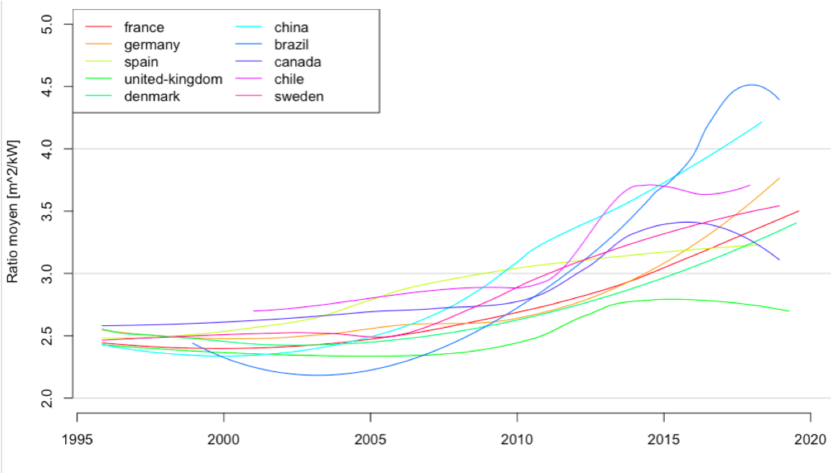Figure 3 – Evolution of the average specific area of wind turbines [$m^2/kW$] by country as a function of the installation date.

System	CAPEX 5% quantile €/kW	CAPEX median €/kW	CAPEX 95% quantile €/kW	Fixed O&M €/kW/year
Onshore wind	850	1500	1875	40

System	CAPEX China €/kW	CAPEX Europe €/kW	Fixed O&M €/kW/year
Offshore wind	2500	3300	75

For onshore wind, LCOEs between €50 and €70/MWh are found, which corresponds to the orders of magnitude found in tender responses, as in 2020 [AOCRE2020], where the average price of selected projects was €62/MWh. The same remark can be made here as in the PV case.

Conclusion

We have given a simple formula for computing the LCOE of a means of electricity generation from annualised costs. For different families of generation, we have discussed the factors affecting costs. These costs can be used to feed a model estimating the costs of the power system, as we did in a previous post [PostPrec]. These data can serve as a basis for our practical exercise on the optimisation and planning of the power system in a context of energy transition (which will be put online as open source shortly). In a future post I will complement this one with economic data for battery storage, flywheels, and power to gas technologies (hydrogen or methane). We will also focus on environmental aspects in another post. Note that the discounting model is far from perfect, but there is no much better one. For very long lifetimes one method is to stop discounting after a certain number of years. My view, no doubt a personal one, is that economic evaluations are necessary and illuminating; one must know how to do them and understand what underpins them, one must carry out sensitivity analyses and step back from the underlying uncertainties. However, reducing decisions as important as those about our energy future to the evaluation of a single indicator seems to me naive. More generally, we think it is also naive to believe that every human activity has an objectively determinable economic cost that could be minimised to move towards an “efficient” society. We have recalled that comparing means of generation economically raises two major difficulties. The first, of a technical nature, requires taking a view of the power system as a whole, such as the one we began in our previous post [PostPrec], since it is obvious that a non-dispatchable MWh does not have the same value as a dispatchable one. The second, economic, requires accounting for all the costs and their timing. We have recalled the classical framework for handling that difficulty. We hope through this post to open a space for discussion in the democratic debate around the energy transition that is scientific, allowing the models and parameters (such as discounting) to be questioned while avoiding comparing things that are not comparable. An approach such as the one applied in [Jancovici2018], which would consist in accounting only for investment costs without accounting for discounting, operating costs, decommissioning costs and marginal costs, is not suited to our objectives. This is a subject that can evolve fairly quickly and on which it is difficult to master everything; we will listen to the remarks and proposals made in the comments. In other words, the data and models proposed here are open to discussion, and we will try to update this post from the constructive comments made and from developments over time.

Finally, the cost of the current fleet discussed in the previous post [PostPrec] will certainly rise, whether in a context of refurbishment or renewal of the nuclear fleet, or in the perspective of developing a renewable + back-up mix. That increase could be substantial, but to put it in perspective one must recall that the cost of electricity generation in the residential sector corresponds to only about 1/3 of the price of electricity. Taxes (about 1/3) and the network use tariff (about 1/3) are added to it. So even if the generation cost went roughly from €50 to €80/MWh, that would only translate into a move from €150 to €180/MWh in the price of electricity at the socket. For the industrial sector things are very different, because network costs and taxes are very low. It seems to me that we must prepare for these increases, give up the myth of cheap and infinite electricity, encourage energy savings, and support large consumers (energy sieves in the residential and service sectors, electro-intensive industry) starting now.

Bibliography

[PostPrec] May 2020, The electricity generation mix – energy and capacity.

[NREL2018] Simple Levelized Cost of Energy (LCOE) Calculator Documentation

[Williams2019] Williams and Tuber, Energy Policy 2019 - Levelised cost of energy – A theoretical justification and critical assessment

[CRE2019] 2019 - CRE report - Coûts et rentabilités du grand photovoltaïque en métropole continentale

[CDC2012] 2012 Les coûts de la filière électro nucléaire

[CDC2014] Le coût de production de l’électricité nucléaire, 2014 update

[CDC2016] 2016 annual public report, Volume I - La maintenance des centrales nucléaires : une politique remise à niveau, des incertitudes à lever

[CDC2019] July 2019 Court of Auditors report on nuclear fuel management

[CDC2020] March 2020 L’arrêt et le démantèlement des installations nucléaires

[IRENA2012] IRENA 2012 - Cost analysis of Hydropower

[RevEnergie2019] LA RÉDUCTION DES COÛTS DE CONSTRUCTION DU NOUVEAU NUCLÉAIRE No. 642 / January-February 2019 - by Michel Berthélemy and Jean-Guy Devezeaux de Lavergne

[Cost2013] Current and Prospective Costs of Electricity Generation until 2050

[EIA2016] Capital costs, U.S. Energy Information Administration, 2016

[Peysson2019] 2019 Pierre Peysson, IMPACT DE LA RÈGLEMENTATION SUR LES COÛTS DE PRODUCTION DE L’ÉOLIEN EN MER EN EUROPE

[Jancovici2018] Jean-Marc Jancovici’s blog, 2018. 100% renouvelable pour pas plus cher, fastoche ?

[ADEMEGES] $CO_2$ emissions balance of coal

Appendices

Appendix 1 - Discount rate, a discussion

Discussing discounting goes far beyond what I can do here today without boring you; it is a whole branch of economics. Let us just note that 8% corresponds to a short-termist view, even though there is worse (some capital managers will want 10% or even 15%), but that even at 4% one does not see much beyond 40 years. Somewhat tense discussions took place on this question around the Stern review on the consequences of climate change (expected at the time to occur far in the future). There are methods that consist in no longer discounting beyond a certain duration, to avoid crushing costs. Even in a “degrowth” world or with zero inflation, discounting can hardly approach zero. This small model and the value of its single parameter raise important societal questions, and we will not shed decisive light on them here. Discounting reflects several elements, and we will mention a few.

The first is inflation. With inflation $\tau_I$, the money $x_{n,n}$ obtained in year $n$ in year-$n$ currency is worth only $x_{n,n+1}=x_{n,n}/(1+\tau_I)$ in year-$(n+1)$ currency. For someone who borrowed the money $x_{0,0}$ in year $0$ and repaid $x_{n,n}$ each year with interest $\tau_N$: $\sum_n x_{n,n}\times (1+\tau_N)^n =x_{0,0}$, the total repayment expressed in year-$0$ currency would be $\sum_n x_{n,0}/(1+\tau_I)^n*(1+\tau_N)^n$. That sum will exceed $x_{0,0}$ only if $\tau_N>\tau_I$. The “real” interest rate $\tau_R=\tau_N-\tau_I$ is classically defined by opposition to the “nominal” rate $\tau_N$, and the following approximation is often made \(\sum_n x_{n,0}/(1+\tau_I)^n*(1+\tau_N)^n \approx \sum_n x_{n,0}\times (1+\tau_R)^n\) One thus easily understands that the nominal discount rate generally has a floor at the level of inflation, and that periods of high inflation, such as the one we experienced in the 1970s, are conducive to crushing investment costs in an LCOE calculation. This played an important role in the construction of the current nuclear fleet. Zero inflation does not necessarily imply zero discounting.

The other important factors are then linked to the real rate $\tau_R$. The analysis of that rate will depend on the capital in our possession that can be dedicated to investment and on the ability to borrow. If one is a company with capital and seeks to draw as much profit as possible from it, the question becomes one of the return on capital (which can be computed at a given time as a function of the maturity and the risk one is willing to take); but the value that can be extracted from capital is also a matter of corporate strategy, and if the aim is to enter a market, crush a competitor, or if strong future growth of the company is expected, a rather low real rate will be chosen. If one does not own the capital in question, the rate may reflect a combination of the interest rates of various bank loans. Thus one can see that an LCOE including a real rate relating to a minimum expected return on investment corresponds to a purchase tariff requested in a call for tenders. In the case of a contract for difference, as for Hinkley Point, the tariff is indexed on inflation and therefore inflation must not be included in the discount rate calculation.

When discounting a distant expenditure, as for decommissioning or waste management, the underlying reasoning is that the company can set aside a sum at the beginning of the project (provisioning) for decommissioning, and that this money, if well invested, will earn a sum of money linked to the discount rate. In that case discounting is connected to the return on capital. Nuclear operators are today asked to consolidate the provisioning for decommissioning and waste management through investment in dedicated assets.

When investing in a new means of generation, if the construction time does not allow the borrowed money to be repaid immediately, additional fees must be paid in the form of interest during construction. Investment costs $C_I$ should incorporate this aspect, and shorter construction times can in many cases help lower costs. This is a very important subject for the nuclear industry RevEnergie2019. Assuming that a sum $C_{I0}$ is spent uniformly over a construction time $L_I$, with a discount rate $r$, one should be able to recover $C_I$ (investment cost at the date when the plant starts producing) from the formula: \(C_I= C_{I0} * \frac{L_I^{r}}{L_I}, \;\; \text{ where } L_I^{r}= \sum_{n=1}^{L_I}(1+r)^n= \frac{1+r}{r}((1+r)^{L_C}-1)\) In the next appendix, we give a table for $L_{I,r}/L_I$ as a function of $r$ and $L_{I}$, the construction time (the second table in the appendix). One can see there that a construction time of 15 years corresponds to a doubling of investment costs.

Appendix 2 - Table for the corrected lifetime

Table of $L_r$ as a function of the lifetime $L$ and of $r$.

	1E-04	0.01	0.02	0.03	0.04	0.05	0.06	0.07	0.08	0.09	0.1
15	14.99	14.004	13.106	12.296	11.563	10.899	10.295	9.745	9.244	8.786	8.367
20	19.981	18.226	16.678	15.324	14.134	13.085	12.158	11.336	10.604	9.95	9.365
25	24.97	22.243	19.914	17.936	16.247	14.799	13.55	12.469	11.529	10.707	9.985
30	29.957	26.066	22.844	20.188	17.984	16.141	14.591	13.278	12.158	11.198	10.37
35	34.941	29.703	25.499	22.132	19.411	17.193	15.368	13.854	12.587	11.518	10.609
40	39.922	33.163	27.903	23.808	20.584	18.017	15.949	14.265	12.879	11.726	10.757
45	44.901	36.455	30.08	25.254	21.549	18.663	16.383	14.558	13.077	11.861	10.849
50	49.878	39.588	32.052	26.502	22.341	19.169	16.708	14.767	13.212	11.948	10.906
55	54.852	42.569	33.838	27.578	22.993	19.565	16.95	14.916	13.304	12.005	10.942
60	59.823	45.405	35.456	28.506	23.528	19.876	17.131	15.022	13.367	12.042	10.964
65	64.792	48.103	36.921	29.306	23.969	20.119	17.266	15.098	13.409	12.066	10.978
70	69.759	50.67	38.249	29.997	24.33	20.31	17.368	15.152	13.438	12.082	10.986
75	74.723	53.113	39.451	30.593	24.628	20.459	17.443	15.19	13.458	12.092	10.991
80	79.685	55.437	40.539	31.107	24.872	20.576	17.5	15.218	13.471	12.099	10.995

Table for $L_{I,r}/L_I$ as a function of $r$ and $L_{I}$, the construction time.

	0.02	0.04	0.06	0.08	0.1
1	1.020000	1.040000	1.060000	1.080000	1.100000
2	1.030200	1.060800	1.091800	1.123200	1.155000
3	1.040536	1.082155	1.124872	1.168704	1.213667
4	1.051010	1.104081	1.159273	1.216650	1.276275
5	1.061624	1.126595	1.195064	1.267186	1.343122
6	1.072381	1.149716	1.232306	1.320467	1.414529
7	1.083281	1.173461	1.271067	1.376661	1.490841
8	1.094329	1.197849	1.311414	1.435945	1.572435
9	1.105525	1.222901	1.353422	1.498507	1.659714
10	1.116872	1.248635	1.397164	1.564549	1.753117
11	1.128372	1.275073	1.442722	1.634284	1.853117
12	1.140028	1.302237	1.490178	1.707941	1.960226
13	1.151841	1.330147	1.539621	1.785763	2.074999
14	1.163815	1.358828	1.591141	1.868008	2.198034
15	1.175952	1.388302	1.644835	1.954952	2.329982

Appendix 3 - Additional material on nuclear

Appendix 3-a. Decommissioning and nuclear waste management.

Assessing the provisions for decommissioning and waste is a delicate task whose ins and outs are fairly well explained in two Court of Auditors reports, on nuclear fuel management [CDC2019] and on the decommissioning of installations [CDC2020]. These reports follow the more general reports [CDC2012] and [CDC2014] on the cost of nuclear. To understand the figures given in these reports, for decommissioning as well as for waste management, one must distinguish between:

Moreover, one must distinguish the sums allocated to EDF from those allocated to ORANO and the CEA. Let us assume (debatably) that those allocated to EDF are exactly those linked to nuclear electricity generation, and let us relate the sums given in euros to the installed capacity of 63 GW so as to obtain amounts in [€/kW] and [€/kW/year] (easier to interpret with respect to the rest of this post).

As regards decommissioning, €18.5 bn of gross charges are mentioned ([CDC2020] p103). That is less than €300/kW of gross charges related to installed capacity; the Court of Auditors asks for further analysis, and the decommissioning operations to come will no doubt strengthen the assessment method. In [CDC2020] p117 the amounts provisioned by EDF for decommissioning nuclear generation installations between 2013 and 2018 are given. Taking an average and relating it to installed capacity, one arrives at €8/kW/year. The corresponding provisioning schedule follows from an assumption about the evolution of the fleet judged somewhat too optimistic by the Court of Auditors (see [CDC2020] p118).

For waste management, one can deduce from what is written on p89-90 of the report [CDC2019] that in 2017 all these gross charges for waste management represented for EDF about €45 bn before discounting and €20 bn after discounting. That includes in particular the Cigéo project (€25 bn before discounting), for which the Court encourages a reassessment of costs, already discussed in the 2012 report [CDC2012] p84. Related to the generation fleet, that means a little more than €700/kW, reduced to about €310/kW “today” when discounting is taken into account. Note that we give these amounts relative to installed capacity, whereas they should rather be related to the energy produced so far, or produced over the lifetime of the installations. Note that these charges relate to future costs and do not include past investments already amortised. For provisioning, the 2014 report gives a value of €1.2 bn in 2013, i.e. €19/kW/year [CDC2014].

Sensitivity of the results. In every case these provisions depend on:

For waste, these provisions also depend on many parameters relating to the future evolution of the fuel cycle, on which the Court of Auditors encourages clarification:

Appendix 3-b. Costs of a major nuclear accident

At present, the costs of insurance against a possible accident are not really integrated, since the corresponding insurance is capped. An assessment is proposed by IRSN, for a cost of €420 bn in the case of a major accident in France. Another study gives a cost of €120 bn (the one used by the Court of Auditors in its reports). It seems very glib to want to associate a probability with this type of event, but one can for instance say that 400 GW of nuclear have been installed worldwide with an average operating duration of around 30 years. That has led to two major accidents, which suggests assigning to the cost of a major accident a weight of $1.6*10^{-10}/kW/year$, i.e. €70/kW/year. That assessment does not account for how insurance works, nor for the investment of the contributed money, which could greatly reduce this value. That is what is done in [CDC2014] , and it gives negligible sums, at worst a few €/MWh. Determining this weight and the associated cost raises many questions; the Court of Auditors’ report proposes another approach with a weight of 1 over the whole French fleet and a cost of €120 bn. Reading Jean-Pierre Dupuy’s book “Pour un catastrophisme éclairé” is interesting on the subject of large cost / small weight; it prefigures the notion of the black swan developed later in the world of finance. In any case, insurance cost is not the source of an explosion in costs and, even though it is not negligible either, we will not take it into account here. Note nonetheless that reducing this cost to a simple economic cost seems to us a limited approach.